Chapter 22
Hyperspectral

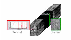
An hyperspectral image contains a collection of spectral pixels or equivalently, a collection of spectral bands.

An hyperspectral system 22.1 acquired radiance, each pixel contains fine spectral information fine that depends of:

• Spectrum of the light source (in practice, the sun) and atmospheric disturbances.
• Spectral responses of different materials in the overlap zone and of the nature of the mixture.

Preliminary treatments allow to perform atmospheric correction for estimating a reflectance cube spectral by subtraction of information extrinsic of the scene (see also 12.2).

22.1 Unmixing

22.1.1 Linear mixing model

Reflectance information depends only of the materials spectral responses in the scene. When the mixture between materials is macroscopic, the linear mixing model of spectra is generally admitted. In this case, the image typically looks like this:

We notice 22.2 the presence of pure pixels, and pixel-blending. The LMM acknowledges that reflectance spectrum associated with each pixel is a linear combination of pure materials in the recovery area, commonly known as “”endmembers. This is illustrated in 22.3

The “ left” term represents the different spectral bands of data cube. The “ right” term represents a “ product” between the reflectance spectra of endmembers and their respective abundances. Abundance band of endmembers is image grayscale between 0 and 1. The pixel i of the abundance band of endmember j is s_ji. This value is the abundance of endmember j in the pixel i. Under certain conditions  [62], this value can be interpreted as the ratio surface of the material in the overlap zone (22.2). In practice, one can reasonably expect that:

• a limit number of pure materials compose the scene.
• the scene contains pure pixels if the spatial resolution is sufficient and do not necessarily contains them otherwise.

Many techniques of unmixing in hyperspectral image analysis are based on geometric approach where each pixel is seen as a spectral vector of L (number of spectral bands). The spectral bands can then be written as vectors.

By deduction of 22.3 et de 22.4, the LMM needs to decompose R as:

J is the number of endmembers and the number of spectral pixels I:

• J columns of the matrix A contain the spectra of endmembers.
• J rows of the matrix S contain the abundance maps vectorized, we call the columns vectors of abundances of matrix S.
• The matrix N, of dimensions LXI is a matrix of additive noise.

The unmixing problem is to estimate matrices A and S from R or possibly of Ẍ, an estimate of the denoised matrix signal.

Several physical constraints can be taken into account to solve the unmixing problem:

• C1: reflectance spectra are positives (non negative matrix A).
• C2: positivity abundances are positive (non-negative matrix S).
• C3: additivity abundance (the sum of the coefficients of each column of the matrix S is 1).
• Independence between the “algebraic spectral vectors” of endmembers associated with linearity and mixtures of spectra, so that the simplex property described in paragraph below.

22.1.2 Simplex

Recent unmixing algorithms based on the “property of simplex.” In a vector space of dimension J -1, we can associate to J vectors algebrically independent, J points which define the vertices of a J-simplex 22.5.

Hyperspectral cube of L bands, based on J endmembers, may be contained in a affine subspace of dimension J -1. A relevant subspace in the sense of signal-to-noise ratio is generally obtained by Principal Component Analysis (PCA) 14.7. In practice, the J -1 eigenvectors associated with highest values are the columns of a projection matrix V of dimension (Lx(J -1)). Reduced data Z, of dimensions ((J -1)xI) are obtained by the operation: Z = V^T ()

where each column of where the average spectrum is subtracted, generally estimated under maximum likelihood. In the subspace carrying the column-vectors Z, endmembers spectra oare associated to the top of the simplex. If the noise is negligible, the simplex circumscribed reduced data.

This property shows that the endmembers research are the vertices of a simplex that circumscribes the data. However, an infinity of different simplices can identify the same data set. In fact, the problem of unmixing generally does not have a unique solution. This degeneration can also be demonstrated by the formalism of the non-negative matrices factorization [3].

It is therefore necessary to choose the most physically relevant solution. All unmixing techniques based on this simplex property admit that the best solution is defined by the allowable minimum volume simplex, or the notion of volume is extended to all finite dimensions (possibly different from 3).

22.1.3 State of the art unmixing algorithms selection

The more recent linear unmixing algorithms exploit the simplex property. It is possible to classify these methods into several families:

22.1.3.1 Family 1

A first family of unmixing algorithms are based on research of the endmembers “among” data. This means that a minimum of one pure pixel must be associated with each endmembers. If this hypothesis is not verified, it will produce an estimation error of the endmembers spectra. The historical advantage of these algorithms are their low algorithmic complexity. The three best known are :

• PPI (Pixel Purity Index)
• VCA NFINDER (Vertex Component Analysis) [96]

In addition to its success recognized by the community and very competitive algorithmic complexity, the endmembers estimation is unbiased in absence of noise (and when there are pure pixels).

VCA The VCA algorithm is systematically used to initialize various studied algorithms (except MVES, based on a different initialization).

Important elements on the operation of VCA:

• The VCA algorithm is based on iterative projections of the data orthogonal to the subspace already held by the endmembers.
• Biaised when degree of purity is lower than 1.

22.1.3.2 Family 2

A second family is composed of algorithms which are looking for the simplex of minimum volume circumscribing the data. Phase initialization consists in determining an initial simplex any circumscribing the data. Then, a numerical optimization scheme minimizes a functional, increasing function of the volume generalized, itself dependent of estimated endmembersin the current iteration. The optimization scheme is constrained by the fact that the data have remained on the simplex and possibly by constraints C1, C2 and C3.

Existing algorithms are:

• MVSA (Minimum Volume Simplex Analysis) [87].
• MVES (Minimum Volume Enclosing Simplex) [Chan2009].
• SISAL (Simplex Identification via Split Augmented Lagrangian) [13].

Main differences between algorithms are:

• The numerical optimization scheme.
• The way constraints are taken into account.

These issues impact the computational complexity and the precision of the estimation.

MVSA [87] MVSA key points:

• Initialization by VCA.
• All spectral pixels included in the simplex estimate (approximatively) by VCA does not impact the constraint of data to belong to the researched simplex, they are simply delete the data used in the minimization of the simplex to reduce the algorithmic complexity.
• The highly developed optimization technique uses sequential quadratic programming (Sequential Quadratic Programming - SQP) and more specifically of the category “Quasi-Newton”under constraint.

MVES [23] MVES key points:

• Initialization by non-trivial iterative method (LP Linear Programming for Linear Programming), different from VCA.
• Resolution of problem by LP.

SISAL [13] SISAL key points:

• Initialisation by VCA.
• Selection of similar spectral pixels as MVSA to reduce computational complexity.
• Advanced optimization technique combining multiple features.
  • Decomposition of the non convex problem in convex set of problems.
  • Development of a specific method of separation of variables for considering Lagrangian increases with a good design properties.

22.1.3.3 Family 3

Non negative matrix factorization algorithms (NMF for Non-negative Matrix Factorization). The purpose of this branch of applied mathematics is to factor a non-negative matrix, X in our case, into a product of non negative matrices: AS by minimizing a distance between X and AS and with an adapted regularization to lift the degeneration in an appropriate manner adapted to the physical problems associated with unmixing.

MDMD-NMF [63] Key points of MDMD-NMF:

• VCA initialization.
• Minimizing the norm of standard Frobenius with a spectral regularization and a regularization “Space”(the matrix of abundances).
  • Minimum spectral Dispersion: the spectral regularization encourages the variance of coefficients of a spectrum of endmembers to be low.
  • Maximum spatial dispersion: the spatial regularization encourages the vector of abundances to occupy all the admissible parts (more information in [62]). it presents a certain analogy with the minimum volume constraint.

22.1.3.4 Further remarks

Algorithms of families 1 and 2 estimate “ only” the spectra of endmembers. The estimated abundance maps held a posteri and requires the application of an algorithm like Fully Constrained Least Square (FCLS) otb::FCLSUnmixingImageFilter [57]. VSS includes an specific algorithm for the estimation of the abundances. The unmixing is a general non-convex problem, which explains the importance of the initialization of algorithms.

Overview of algorithms and related physical constraints:

22.1.3.5 Basic hyperspectral unmixing example

The source code for this example can be found in the file
Examples/Hyperspectral/HyperspectralUnmixingExample.cxx.

This example illustrates the use of the otb::VcaImageFilter and otb::UnConstrainedLeastSquareImageFilter . The VCA filter computes endmembers using the Vertex Component Analysis and UCLS performs unmixing on the input image using these endmembers.

The first step required to use these filters is to include its header files.

We start by defining the types for the images and the reader and the writer. We choose to work with a otb::VectorImage , since we will produce a multi-channel image (the principal components) from a multi-channel input image.

We instantiate now the image reader and we set the image file name.

For now we need to rescale the input image between 0 and 1 to perform the unmixing algorithm. We use the otb::VectorRescaleIntensityImageFilter .

We define the type for the VCA filter. It is templated over the input image type. The only parameter is the number of endmembers which needs to be estimated. We can now the instantiate the filter.

We transform the output estimate endmembers to a matrix representation

We can now procedd to the unmixing algorithm.Parameters needed are the input image and the endmembers matrix.

We now instantiate the writer and set the file name for the output image and trigger the unmixing computation with the Update() of the writer.

Figure 22.6 shows the result of applying unmixing to an AVIRIS image (220 bands). This dataset is freely available at http://www.ehu.es/ccwintco/index.php/Hyperspectral_Remote_Sensing_ScenesIndian_Pines

22.2 Dimensionality reduction

Please refer to chapter 18, page 777 for a presentation of dimension reduction methods available in OTB.

22.3 Anomaly detection

By definition, an anomaly in a scene is an element that does not expect to find. The unusual element is likely different from its environment and its presence is in the minority scene. Typically, a vehicle in natural environment, a rock in a field, a wooden hut in a forest are anomalies that can be desired to detect using a hyperspectral imaging. This implies that the spectral response of the anomaly can be discriminated in the spectral response of “background clutter”. This also implies that the pixels associated to anomalies, the anomalous pixels are sufficiently rare and/or punctual to be considered as such. These properties can be viewed as spectral and spatial hypotheses on which the techniques of detection anomalies in hyperspectral images rely on.

Literature on hyperspectral imaging generally distinguishes target detection and detection anomalies:

• We speak of detection of targets when the spectral response element of the research is used as input to the detection algorithm. This is an a priori information that can, in theory, allow to construct algorithms with very high detection score, such as for example the Adaptive Matched Filter (AMF) or Adaptive Cosine/Coherence Estimator (ACE). Nevertheless, thin enough knowledge of the researched spectrum is a difficult information to hold in practice, leading the use of anomaly detection algorithms.
• We speak of detection of anomalies (or outliers) when the spectrum of the unusual element is not required by the algorithm. For this reason, we often associate the term “Unsupervised” detection. Nevertheless, these algorithms depend generally of “structural” parameters. For example, in the case of detection on a sliding window, selecting the right dimensions is based on an a priori knowledge of the anomalies size. We focus here on algorithms for anomaly detection.

In 22.7, we introduce some notions that will be useful later. Anomaly detection algorithms have an image as input and consider a map serving as a detection tool for making a decision. A adaptive thresholding provides a estimated mask detection that we hope is the most similar possible as the ground truth mask, unknown in practice.

Two approaches dominate the state of the art in anomaly detection in hyperspectral images. Methods which use Pursuit Projection (PP) and methods based on a probabilistic modelization of the background and possibly of the target class with statistical hypothesis tests. The PP consists in projecting linearly spectral pixels on vectors wi which optimizes a criterion sensitive to the presence of anomalies (like Kurtosis). This gives a series of maps of projections where anomalies contrast very strongly with the background. But the automatic estimation of map detection have also major difficulties, including:

• How many projectors should I consider?
• What (s) projector (s) to choose?
• How to manage an inhomogeneous background?
• Detection performances varies with the spatial dimensions of the image (number of samples)
• These algorithms usually do not have a structure allowing parallelization
• These algorithms do not generally have a “constant false alarm rate”.

Algorithms described here are RX (presented in the first version in [114] and GMRF [122]. They are based on probability models, statistics and hypothesis tests and sliding window. These approaches consist in answering the following question : “The pixel (or set of neighboring pixels) tests looks like background pixels?”, by a process of test statistics. More fully, this approach requires:

• A model for the background
• The choice of a statistic test
• Eventually, a model for the class “anomaly”
• Estimators for the parameters a priori unknown
• Hypothesis of homogeneity for a satisfactory compromise between:
  • The number of samples compared to the number of estimate parameters
  • The homogeneity, including the background
  • Algorithmic complexity (although the algorithms considered are highly parallelizable)

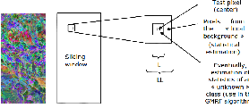
Principle of RX and GMRF can be resume with 22.8.

An optional first step is to reduce the size of spectral data while maintaining information related to anomalies. Then, the spectral pixels are tested one by oneturn (parallelizable task). The pixel test works on a sliding window (see 22.9). This window consists of two sub windows, centered on the pixel test of dimensions L and LL, with L < LL.

• Pixels belonging to the annulus formed the class “local background”. The statistical parameters of the background, required by statistical tests, are estimated from these spectral pixels. One of the challenges is to find a compromise on the thickness of the annulus (and therefore the number statistical sampling) where:
  • If the annulus is too thick, the local background is no longer homogeneous
  • If the number of samples is too low, the precision of the statistical estimation of the model parameters for the background is too low
• Pixels of the central part of the sliding window belong to the class “unknown”. If the test pixel (central pixel) is an anomaly, it is possible that its neighbors pixels are also anomalies, which imply to not to choose a too small value for L if it is known that anomalies can be distribute over several pixels.

Once all the parameters are estimated, a statistical test is performed and assigns a value Λ(i) to the tested pixel i. A map of detection is thus formed.

The RX algorithm is available in OTB through the otb::LocalRxDetectorFilter class.